Table of Contents
Calibration curve
Despite the use of a common set of laboratory protocols, the dose calibration curves produced from each laboratory are unique and may produce different dose estimates 1). To determine DC counts and ensure internally consistent dose estimates, test samples and calibration curves from the same laboratory should both be processed using ADCI software. A calibration curve is required to perform dose estimation.
Generation of curve
The curve calibration wizard guides users through the necessary steps to generate a curve from a set of processed samples. While using the wizard, dose and response data are automatically populated based on the combination of selected processed samples and SVM sigma value, streamlining the data-entry process. The steps within the wizard can also be performed manually if desired, those steps are described below.
Generate curve based on processed calibration samples
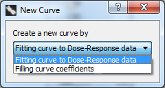
This curve generation method requires processed samples. Click the ![]() icon and select “Fitting curve to Dose-Response data” from the dropdown list presented within the dialog box and click “OK”.
icon and select “Fitting curve to Dose-Response data” from the dropdown list presented within the dialog box and click “OK”.

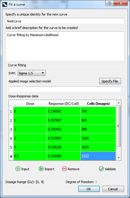
- Specify an unique identify for the new curve
A name for the curve to be created. This identifier will appear under “Curve identity” within the list of curves in the main GUI. - Add a brief description for the curve to be created
This description will appear in the console when the curve is highlighted within the list of curves in the main GUI. - SVM
The SVM sigma value should match the SVM sigma value of the you wish to use for future dose estimation using this curve. Please view the sigma value page for recommended sigma values to select. - Applied image selection model
The image selection model selected here should match the image selection model chosen during future dose estimation. - Input Response-Dose data to create a curve
At least three samples must be input to the dose-response list. For each sample, both dose and response must be input. To add a new sample click “Import”, select the appropriate calibration sample and SVM Sigma value, and a new entry will appear the dose-response list. Dose is represented in Gray (Gy) units and is known based on the exposure of the calibration sample. For example, if a calibration sample was exposed to radiation at 2 Gy, 2 should be entered in the dose field. The “Import” functionality automatically retrieves DC/Cell of the sample at the specified SVM Sigma value.
Double clicking dose or response fields allows the field to be edited if necessary. For each sample to be edited, double click on the dose or response column, which will select the text to be changed. Anything typed while the field is selected will overwrite what was previously present. This process may be repeated in order to edit fields as necessary.
If desired, all fields can be entered manually by clicking “Input”. Response (DC/Cell) can be found in the console after clicking a processed sample in the sample list within the main GUI. DC/Cell values are present for sigma values in the range 0.8 to 1.8. The appropriate DC/Cell value to enter corresponds to the SVM sigma value you have chosen to use. Dose-response entries can be removed by clicking a dose-response row and clicking “Remove”.
After entering or importing all desired dose-response entries, “Validate” must be clicked before the “OK” button will be enabled. “Validate” ensures the contents of the Dose-Response list are numeric and are greater than zero.
- Click “OK” and save curve
The curve is now created and has been added to the workspace. If you would like to save the curve for future use after the current session, you can save it now. Alternatively, it can be saved later by clicking the icon.
icon.

Generate curve by manually entering curve coefficients
It is not recommended to enter curve coefficients if you intend to process test samples using ADCI software. If you enter curve coefficients, we recommend you also manually enter DC frequencies for dose estimation from a manual count of DCs. If a sample is processed using ADCI software it has an associated SVM sigma value. Higher SVM sigma values find more DCs than lower SVM sigma values but still generally underestimate DC counts when compared to expert manual examination2). Manual counts of DCs are of course not associated with any SVM sigma value. Therefore, entering curve coefficients generated from a manual count of DCs and performing dose estimation on a sample processed by ADCI software will not generate results accurately.
This curve does not require processed calibration samples. This option is meant for labs which have previously calculated calibration curves and have access to those curve coefficients. Please take note of the above warning when considering this curve generation option. To manually enter curve coefficients, click the ![]() icon and select “Filling curve coefficients” from the dropdown list presented within the dialog box and click “OK”.
icon and select “Filling curve coefficients” from the dropdown list presented within the dialog box and click “OK”.

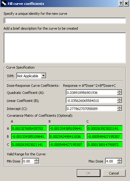
- Specify an identify for the curve to be created
A name for the curve. This identifier will appear under “Curve identity” within the list of curves in the main GUI. - Add a brief description for the curve to be created
This description will appear in the console when the curve is highlighted within the list of curves in the main GUI. - SVM
In almost all cases, SVM should be left to read “Not Applicable” when creating a curve by manually entering coefficients. As described in the warning above, the SVM sigma value is related to how many dicentric chromosomes are found when a sample is processed. If a curve was previously created independently of ADCI software, SVM is not applicable. An SVM should be selected if you are entering curve coefficients from a curve you have previously created using ADCI software, however note it is more straightforward to simply save a curve generated by ADCI software instead of re-entering coefficients in this manner. - Curve coefficients (A,B, and C)
Three curve coefficients are defined as:A*Dose^2+B*Dose+C
Enter values under the headings “Quadratic Coefficient (A)”, “Linear Coefficient (B)”, and “Intercept (C)”.
- Covariance Matrix of Coefficients (Optional)
A covariance matrix can optionally be entered here. As values in the covariance matrix are symmetric, repetitive values are populated automatically. The presence of a covariance matrix allows curve confidence intervals to be calculated and allows ADCI to take uncertainty based on this calibration curve into account during dose estimation. Note if a covariance matrix is not supplied, uncertainty based on the Poisson nature of dicentric yield can still be taken into account during dose estimation if requested. - Valid Range for the Curve
ADCI software will not attempt to accurately report estimated dose of a test sample outside the “Min Dose” and “Max Dose” range. The minimum and maximum physical dose (in Gy) present in calibration data should be entered in “Min Dose” and “Max Dose” fields respectively. If dose is estimated using a test sample with estimated dose outside the Min Dose and Max Dose range, the software will report the test sample has estimated dose > Max Dose or < Min Dose. - Click “OK” and save curve
The curve is now created and has been added to the workspace. If you would like to save the curve for future use after the current session, you can save it now. Alternatively, it can be saved later by clicking the icon.
icon.

Import an existing curve
To import a curve which has previously been saved, click the ![]() icon. A dialog will appear allowing you to select curves from the file system. Saved curves have the file extension adcicurve.
icon. A dialog will appear allowing you to select curves from the file system. Saved curves have the file extension adcicurve.
Curve fitting method
The following curve fitting methods can be selected through [Settings (menu bar) → Statistics Options → Curve Fitting Settings]:
The Maximum-Likelihood Method is recommended by IAEA and is the default curve fitting method. Note if the curve fitting method is changed, a new curve must be generated for the setting to take effect. Curves generated in the past will not be updated to the new method.
Visualization of curves
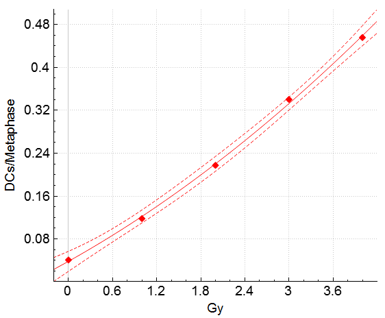
Calibration curves can plotted within the plot display section of the main GUI. All plots can be magnified to view specific intervals. Instructions on how to do this can be found on the plots information page of this wiki.
Confidence intervals
When generating a calibration curve plot, 95% confidence intervals (CI) may optionally be displayed. The following setting: [Settings (menu bar) → Statistics Options → Display calibration curve 95% CI], controls whether CIs appear when plotting calibration curves. Note this setting controls only whether confidence intervals are displayed. Another option within the same menu [Dose estimation calculates 95% CI due to the curve, if applicable] sets whether curve CI are taken into account during dose estimation.

Curve fitting statistics
Curve fitting stats can be found in the console when a curve is highlighted within the main GUI and are also present in calibration curve reports. These statistics can be used to evaluate curve “goodness of fit”. Available curve fitting statistics are:
Calibration curve degrees of freedom is: n - 3 where n is the number of calibration samples used the generate the curve.